Trumpland and Clinton Islands

Clinton islands.png

It’s informative to display how small of the country, by area, Hilary Clinton won in the 2016 Presidental Election. Above is a map of the regions of the country Hilary won (Clinton Islands) and below is the area of the country Trump won (Trumpland). Given the area difference alone, it appears that Trump won in a landslide, however, in fact, he lost the popular vote by more than 2% to Clinton! This is due to the large differences in population density each candidate won – put simply, Clinton won in the cities and Trump won in the rural areas. The highest percentage Trump supporting region was the central plans while the largest Clinton supporting regions were the San Francisco Bay Area and eastern seaboard running from Washington DC to Boston.

Trumpland.png

US Income Inequality 1970-2010

Screen Shot 2016-12-01 at 4.35.57 PM.png

There is increased attention focused on US income inequality in recent years. It remains a challenge to isolate different contributing factors for this inequality growth over the past generation although some reasons have been cited, such as: increased trade with developing countries, increased income for those with university degrees (only around 30% of the US population), increased role of technology in the economy, etc. This post will not dive into trying to uncover why income inequality is happening, but rather, how the various income groups have been affected since 1970.

Above is a chart displaying the US population grouped into five income brackets. What is clear from the data is for the bottom 80% of US income earners, all groups are receiving a smaller share of total US income than compared to 1970 and 1990. Meanwhile, across this same period, the highest fifth of income-earners in the US have received an increasing share of income compensation – from 43.3% in 1970 to 46.6% in 1990 to 50.3 percent in 2010.

Although, to play devil’s advocate, what makes this issue even more complicated is that individuals are not in the same group over time, it is hard to factor in changes in the quality of goods, or even, the modern luxuries of goods that didn’t even exist 40 years ago such as the internet, smart phones, laptop computers, etc. Even though the percentage of income the bottom 80% of income earners is responsible for has decreased over the period, it’s clear that they are living better lives considering all the improvements in technology, safety, and healthcare.

US Income Distribution 2015

Screen Shot 2016-12-09 at 10.25.56 PM.png

Income data from the 2015 US census reveals some insight. 39% of all households had two or more income earners resulting in 25% of households having a combined income above $100k. Meanwhile, only 9% of US workers (population age 15 or older) have individual incomes over $100k. These high earners are typically associated with high education levels as half of all people with graduate degrees are also among the top 15% of income earners (individual incomes greater than $75k).

In 2015, US median personal income was $30k and the mean personal income was $44k. For the US population aged 15 and above, 43% make less than $25k, 70% make less than $50k, 84% make less than $75k, and 91% make less than $100k. Similar data is displayed in the bar chart above – one chart shows the distribution for ages 25 through 64 and the other for ages 25 and above.

Who Moves? Who Stays?

Screen Shot 2016-12-15 at 10.52.43 PM.png

Recent data from the Pew Research Center gives insight into the demographic profile of US citizens and their moving behavior relative to age, location, and education level. Some highlights: 37% of people have never lived outside their hometowns, 57% of adults have never lived outside their home state, and on the opposite side of the spectrum, only 15% of people have lived in four or more states. The effect of college is a significant difference between ‘movers’ and ‘stayers’ – 77% of college graduates have changed communities at least once compared to only 56% for high school graduates.

The above graph shows the age profile for movers. Most movers are between the age of 18 and 35. There is an initial peak at 18 years old as a large portion of people leave high school for college and there is an even higher peak for movement post college graduation. The most likely age someone will move is around 24 years old – about 37% of people change locations at this age. The graph below shows the net regional US migration patterns in 2007. The South and West are making the largest population gains at the expense of the Northeast and Midwest.

Screen Shot 2016-12-15 at 10.55.40 PM.png

Bay Area Median Home Price 2016

Bay Area Median home price 2016.png

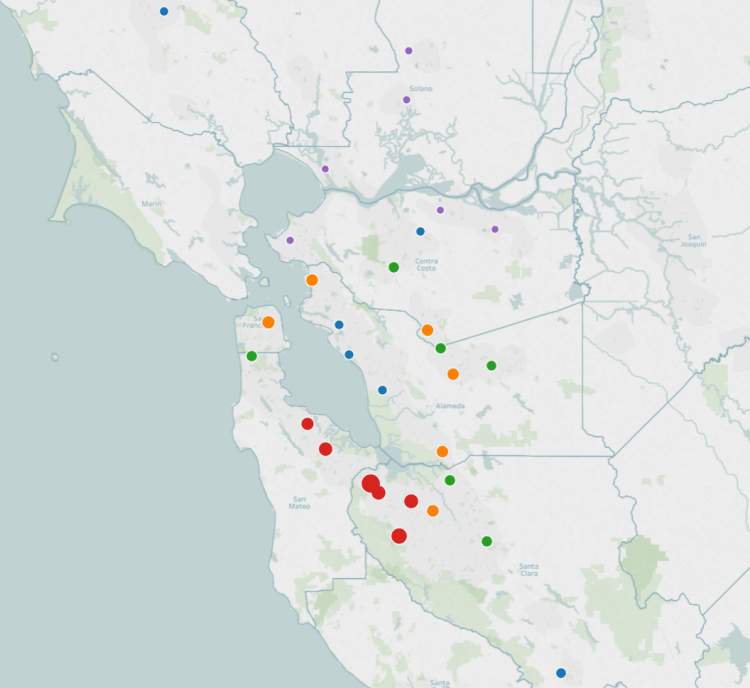
The San Francisco Bay Area is one of the most expensive places to live in the United States. The map above displays the median home price for the top 30 most populated cities in the Bay Area. The larger the bubble, the higher the median home price. The bubbles are also color coded – Red the highest 20%, Orange the next 20%, then Green, Blue, and Purple the lowest 20% by median home price.

Regionally, the cities comprising Silicon Valley are the most expensive and the cities in the northeastern bay are the cheapest. In order, the most expensive cities in the bay area by median home price (via Zillow) as of 2016: Palo Alto at 2.5 million, Cupertino 1.8 million, Mountain View 1.4 million, Sunnyvale 1.4 million, Redwood City 1.3 million, San Mateo 1.1 million, and San Francisco 1.1 million.

The most affordable housing in the Bay Area (of the top 30 by population) are: Richmond 411k, Vacaville 391k, Fairfield 390k, Antioch 364k, Pittsburg 357k, and Vallejo 326k.

Canada’s Immigration

Canada immigration.png

Above is a graphic displaying Canada’s foreign-born population by decade ranging from 1871 through 2011. The size of the bubbles below the graphic display the number of total migrants arriving in millions by decade. Broadly speaking, Canada’s immigration has occurred in three waves. First, a British Isles majority wave from 1871 till the mid-1900’s,  second, a European majority wave from the mid-1900’s through 1990, and third, an Asian majority wave from 1990 running through the present.

Congress and President

Congress and President.png

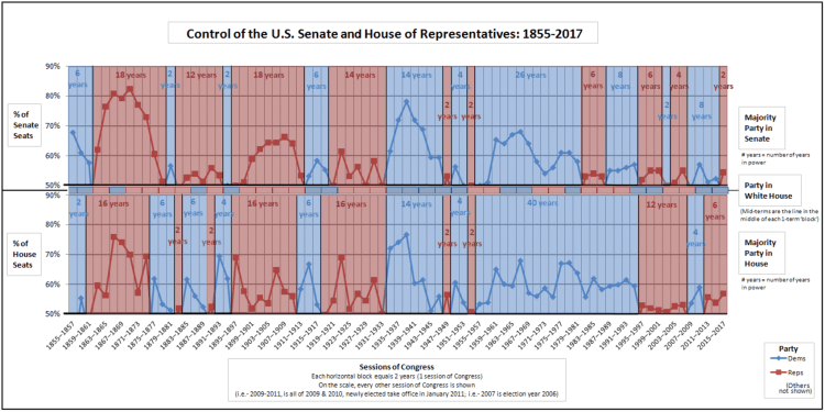
Not only did Donald Trump win the 2016 presidential election, but both the House of Representative and the Senate are majority controlled by the Republican party. Above is a chart displaying which party has controlled congress and the presidency running back through 1855. The Senate is the top chart, the House is the bottom chart, and presidential party in office is the middle color strip between the two. The color indicates which party controlled each branch of congress and the height of the bars in each chart indicate what percentage the controlling party had in those years. Since the great depression, congress has been mostly controlled by the Democrats – having the majority of seats in both the Senate and House for 62 years out of the 84. Since the 1990’s, control in congress has narrowed between the two parties and control as flipped back-and-forth more often than in the previous periods. The 2017 version will feature Republican control in all three for the first time since President Bush II in 2008.

Voter Demographics 2016

Screen Shot 2016-11-19 at 9.43.36 PM.png

Above is a graphic displaying the Republican share of the two-party votes relative to square miles per voter (i.e. population density). As expected, Democrats won a larger fraction of urban areas, on average, while Republicans won more rural areas. Democrats also won a larger share of college graduates, all be it a slim margin 49% to 45%, but won by a substantial margin in both non-white college graduates and the non-white non-college graduate population – 71% and 75% respectively.

Below is a graphic displaying the percentage change in voting behavior for various demographic groups compared to the 2012 election. Trump won a larger percentage of votes in all categories (including Male, White, Black, Hispanic, and Asian) except for Women voters who voted by a 1% larger margin for Hillary than for Obama in 2012.

Screen Shot 2016-11-19 at 9.42.05 PM.png

Electoral College Vs. US Population

EC vs Pop map.png

Hilary Clinton won the popular election 47.7% to 47.4% despite losing the electoral college by a wide margin to Donald Trump. This is only the second time since 1888 that a candidate has won the popular vote, but not the election. This situation has lead some to question if the electoral college system is really the best way to select a president. Liberals claim that it is not fair as large, densely populated states have proportionally less say then less populated rural states that have a minimum 3 electoral votes regardless of population. This claim was interesting, so I decided to investigate further.

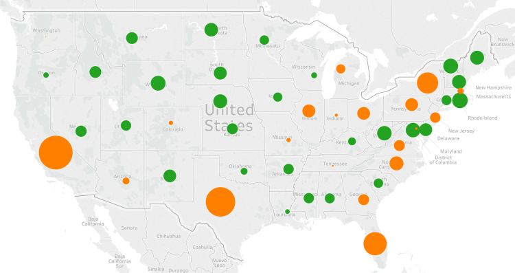
Above is a map displaying the relative difference among the states regarding their ‘over representation’ or ‘under representation’ given population. Orange colored bubbles mean the state has a higher fraction of US population than the fraction of electoral college votes. For example, California has 12.2% of US population, yet only 10.2% of electoral college votes. This is also the case for Texas (8.5% of population verse 7% of electoral college) and likewise for all other orange colored states. The size of the bubble signals a larger margin of under representation.

On the other end of the spectrum, the green colored bubbles mean the state has a higher fraction of electoral college votes compared to their fraction of US population. For example, Wyoming has 0.18% of US population yet has 0.56% of the electoral college – that is, 3 votes out of 538. Again the larger the green bubble signals a wider margin between electoral college votes compared to relative population.

The smaller the bubbles, whether green or orange, means that state was very close to proportional representation between the electoral college and population. For example, Washington state had 2.2% of US population and 2.2% of electoral college votes.

Comparing how the 18 most over represented states voted results in 9 Republican and 9 Democratic states. That is, for every rural over represented Republican state like Wyoming, Alaska, and North Dakota – there are an equal number of small over represented Democratic states like Vermont, Washington DC, and Delaware. To claim the election was lost due to under populated Republican states is inaccurate. The election was won in the battle ground, medium sized swing states of Ohio, Michigan, Wisconsin, and Pennsylvania – all of whom voted Republican this year instead of Democratic was they did in 2012 and 2008.

Screen Shot 2016-11-13 at 5.27.51 PM.png

Above is a table of the 18 most over represented states by electoral college votes. The ‘Elect Diff’ column is the difference between the electoral college percentage minus the US population percent the state has. The ‘Demo16’ column is the Democratic vote percentage, ‘Rep16’ is the Republican vote percentage, ‘Other16’ is the sum of third party vote percentage, and ‘D-R Spread’ is the Democratic vote percentage minus the Republican vote percentage.

US Median Home Price 2015

Median home price map 2016.png

Above is a map of the top 100 metropolitan areas by population in the United States colored and sized according to the median home price. The larger the bubble, the higher the house price. Also, there are color tiers – Red the highest, Orange upper-mid, Green middle, Blue lower-mid, and purple lowest. The national average home price was $215,000.

In 2015, the metro area with the highest median home price is San Jose, CA at $900,000, followed by San Francisco-Oakland at $850,000, Los Angeles at $590,000, New York City at $585,000, and Oxnard at $507,000. The five lowest metro areas by median home price were Akron, OH at $93,000, St. Louis, MO at $89,900, Youngstown, OH at $88,500, McAllen, TX at $85,000, and Dayton, OH at $63,000.