Expensive Cities

rj65zma2r0121.png

It’s tough to compare costs across cities in different countries, but this study tries to do just that. It’s trying to answer the question: What is the average cost of a weeklong holiday trip to selected cities? The question is subject to the predefined assumptions – The trip is for two adults staying in Airbnb, walking & public transit, and doing typical tourist daytime activities like visiting museums, shows, or day-trips.

The graphic above is color-coded by region. The range of costs across cities in the sample fit closely to a normal distribution with the majority of cities falling in the $1000-2000 cost window. Africa and Asia have most of the cheaper cities while Western Europe and Coastal cities in the USA are the most expensive to visit.

Advertisement

California and Canada

Screen Shot 2017-12-11 at 9.52.49 PM.png

Did you know that California (39 million) has more population than Canada (36 million)? The map above displays the area comparison and map below shows how Canada’s population would fit into California. For example, most Canada’s population is concentrated in the two provinces of Ontario and Quebec – these provinces have approximately the same population of southern California. Even though Canada has an area larger than the entire United States, its population can fit into California with room to spare. Side note: California also has a substantially larger economy with a 2.6 trillion nominal GDP compared to 1.5 trillion for Canada (2017).

Screen Shot 2017-12-11 at 9.53.17 PM.png

US City Commute Patterns 2008

Screen Shot 2017-09-04 at 10.47.14 PM.png

Above is a graph displaying the percentage of people that commute by public transit on the x-axis and the percentage commuting by car on the y-axis for various cities around the United States. The size of the bubble relates the workforce population of each city. There doesn’t appear to be a relationship between the size of the city’s population and the percentage of those taking public transit, but if one looks at city density a relationship is clear. Of the top 20 cities in the US by population, the highest density in order are: New York City, San Francisco, Boston, Chicago, Miami, Philadephia, and Washington DC. With exception of Miami (commute data not listed), all of top 6 highest density cities also have the highest fraction of their workforce commuting by public transit.

United States Population Map

Screen Shot 2017-07-31 at 2.52.32 PM.png

As of 2017, the United States population stands at 324 million – the third largest country in the world by population behind India and China. The population ranges across the nation from state to state, from a high of 39 million in California to a low of 585 thousand in Wyoming. The map above distorts each state’s normal area to display its relative population size. In order words, California population represents 12% of the US total and thus takes up 12% of the map, Texas 8.6%, Florida 6.3%, and so on until Wyoming with 0.18%. The states are color coded by groups of ten with the largest ten in red, the next ten in orange, then yellow, light green, and dark green. California and Texas represent 1/5th of US population and the top 5 states make up 37%. The map below is of the United States as normally displayed, with each state relative to it area.

Screen Shot 2017-07-31 at 2.52.36 PM.png

The US in State Highway Shields

Screen Shot 2017-06-09 at 3.16.49 PM.png

If you’re like me, you been across the US and noticed the various State Highway Marker Shields. The above map displays all of them, positioned over each state. Some have historical/social meaning (California – the shape of a shovel (as in digging for gold), Utah – a beehive (a signal of Mormonism), or Pennsylvania – a keystone, as in the Keystone state that connects the east coast to the mid-west), some are merely the outline of the state shape (Idaho, Arizona, Missouri, etc.), and some have no significance at all (Texas, Montana, Illinois, etc.). What’s your sign?

United States Climate Alliance

Screen Shot 2017-07-24 at 9.47.15 PM.png

Even though President Trump withdrew the United States Federal Government from the Paris Agreement on Climate Change, it doesn’t prevent US States or cities from continuing to uphold the agreement. So far, 13 states have committed to Paris Agreement and ~300 cities (including the all of the top 10 largest cities: NYC, LA, Chicago, Houston, Phoenix, Philadelphia, San Antonio, San Diego, Dallas, and San Jose). The map above displays the US states that are currently still in the Paris agreement in blue and the states considering joining the group in green. This group (in blue) made up 32.3% of the US population and 37.6% of US GDP in 2016. Roughly speaking, it can be said that 1/3 of the United States is still part of the Paris Agreement on Climate Change. The map below displays the cities in the agreement (in red) and the USCA in green (as of June 1).

Screen Shot 2017-07-24 at 9.50.03 PM.png

SF Bay Area Median Home Price Apr 2017

Screen Shot 2017-06-02 at 10.20.10 AM.png

Above is a map displaying the median home prices for cities in the SF Bay Area as of April 2017 on Zillow. The most expensive cities in order are: Palo Alto 2.5 million, Cupertino 1.8m, Mountain View 1.5m, Sunnyvale 1.5m, Redwood City 1.3m, San Francisco 1.2m.

Below is a chart displaying the median home price changes for the four largest cities in the Bay Area since Jan 2012. Home prices have doubled in the past five years with cities such as Oakland up 123%, Mountain View up 112%, and Palo Alto up 103% over the period.Screen Shot 2017-06-02 at 10.24.56 AM.png

Bay Area Median Home Price 2016

Bay Area Median home price 2016.png

The San Francisco Bay Area is one of the most expensive places to live in the United States. The map above displays the median home price for the top 30 most populated cities in the Bay Area. The larger the bubble, the higher the median home price. The bubbles are also color coded – Red the highest 20%, Orange the next 20%, then Green, Blue, and Purple the lowest 20% by median home price.

Regionally, the cities comprising Silicon Valley are the most expensive and the cities in the northeastern bay are the cheapest. In order, the most expensive cities in the bay area by median home price (via Zillow) as of 2016: Palo Alto at 2.5 million, Cupertino 1.8 million, Mountain View 1.4 million, Sunnyvale 1.4 million, Redwood City 1.3 million, San Mateo 1.1 million, and San Francisco 1.1 million.

The most affordable housing in the Bay Area (of the top 30 by population) are: Richmond 411k, Vacaville 391k, Fairfield 390k, Antioch 364k, Pittsburg 357k, and Vallejo 326k.

Electoral College Vs. US Population

EC vs Pop map.png

Hilary Clinton won the popular election 47.7% to 47.4% despite losing the electoral college by a wide margin to Donald Trump. This is only the second time since 1888 that a candidate has won the popular vote, but not the election. This situation has lead some to question if the electoral college system is really the best way to select a president. Liberals claim that it is not fair as large, densely populated states have proportionally less say then less populated rural states that have a minimum 3 electoral votes regardless of population. This claim was interesting, so I decided to investigate further.

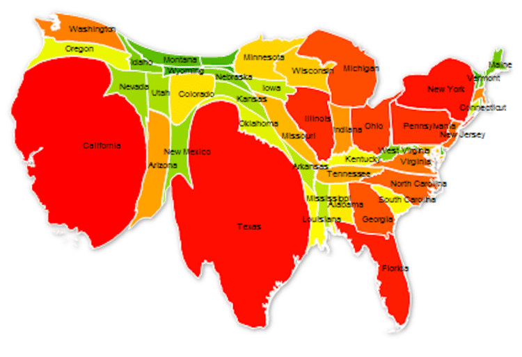
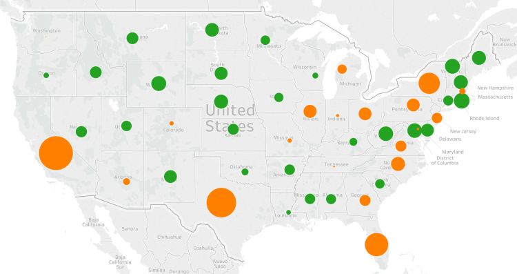
Above is a map displaying the relative difference among the states regarding their ‘over representation’ or ‘under representation’ given population. Orange colored bubbles mean the state has a higher fraction of US population than the fraction of electoral college votes. For example, California has 12.2% of US population, yet only 10.2% of electoral college votes. This is also the case for Texas (8.5% of population verse 7% of electoral college) and likewise for all other orange colored states. The size of the bubble signals a larger margin of under representation.

On the other end of the spectrum, the green colored bubbles mean the state has a higher fraction of electoral college votes compared to their fraction of US population. For example, Wyoming has 0.18% of US population yet has 0.56% of the electoral college – that is, 3 votes out of 538. Again the larger the green bubble signals a wider margin between electoral college votes compared to relative population.

The smaller the bubbles, whether green or orange, means that state was very close to proportional representation between the electoral college and population. For example, Washington state had 2.2% of US population and 2.2% of electoral college votes.

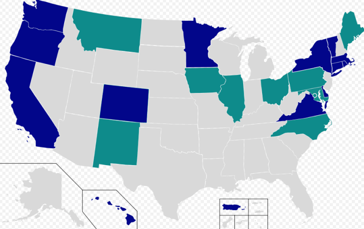
Comparing how the 18 most over represented states voted results in 9 Republican and 9 Democratic states. That is, for every rural over represented Republican state like Wyoming, Alaska, and North Dakota – there are an equal number of small over represented Democratic states like Vermont, Washington DC, and Delaware. To claim the election was lost due to under populated Republican states is inaccurate. The election was won in the battle ground, medium sized swing states of Ohio, Michigan, Wisconsin, and Pennsylvania – all of whom voted Republican this year instead of Democratic was they did in 2012 and 2008.

Screen Shot 2016-11-13 at 5.27.51 PM.png

Above is a table of the 18 most over represented states by electoral college votes. The ‘Elect Diff’ column is the difference between the electoral college percentage minus the US population percent the state has. The ‘Demo16’ column is the Democratic vote percentage, ‘Rep16’ is the Republican vote percentage, ‘Other16’ is the sum of third party vote percentage, and ‘D-R Spread’ is the Democratic vote percentage minus the Republican vote percentage.

US Median Home Price 2015

Median home price map 2016.png

Above is a map of the top 100 metropolitan areas by population in the United States colored and sized according to the median home price. The larger the bubble, the higher the house price. Also, there are color tiers – Red the highest, Orange upper-mid, Green middle, Blue lower-mid, and purple lowest. The national average home price was $215,000.

In 2015, the metro area with the highest median home price is San Jose, CA at $900,000, followed by San Francisco-Oakland at $850,000, Los Angeles at $590,000, New York City at $585,000, and Oxnard at $507,000. The five lowest metro areas by median home price were Akron, OH at $93,000, St. Louis, MO at $89,900, Youngstown, OH at $88,500, McAllen, TX at $85,000, and Dayton, OH at $63,000.